
From Planck to the Modern Atmosphere
The Foundations of Atmospheric Radiation
Tracing the development of radiative transfer theory from Max Planck's quantum revolution and Karl Schwarzschild's atmospheric equations to the modern science of Earth's energy balance.
by Juerg Kaufmann
Introduction — What Does This Chart Actually Mean?
A plain-language guide to understanding Earth's heat radiation and CO₂
The Big Picture
The Earth is constantly receiving energy from the Sun. To stay at a stable temperature, it must radiate the same amount of energy back out into space as invisible infrared heat — the same kind of warmth you feel radiating from a campfire. If something blocks some of that outgoing heat, the planet warms up until a new balance is reached. That "something" is what we call greenhouse gases — mainly water vapour (H₂O), carbon dioxide (CO₂), ozone (O₃), nitrous oxide (N₂O), and methane (CH₄).
Outgoing Longwave Radiation Spectrum
Based on Wijngaarden & Happer — Earth surface at 288 K (15°C)
Reading the Chart — Step by Step
The chart above (recreated from the work of Wijngaarden and Happer) shows how much heat radiation escapes Earth's atmosphere at each frequency of infrared light. Here is how to read it:
The smooth blue curve (~390 W/m²)
This is the theoretical maximum — the heat Earth's surface would radiate if the atmosphere were completely transparent, like a window with no glass. It is calculated using Planck's formula for a surface at about 15°C (288 K).
The green curve (~308 W/m²) — CO₂ = 0 ppm
This shows what happens when you add all greenhouse gases except CO₂. Water vapour, ozone, and other gases already block a significant portion of the outgoing heat. The "bites" taken out of the smooth curve are the frequencies where these gases absorb radiation.
The orange dashed curve (~288 W/m²) — CO₂ = 200 ppm
At 200 ppm CO₂ (a level seen during some glacial periods), the first major "bite" from CO₂ appears around 667 cm⁻¹. This first dose of CO₂ reduces outgoing radiation by about 20 W/m² (from 308 down to 288) — the largest single step.
The purple dashed curve (~282 W/m²) — CO₂ = 300 ppm
At 300 ppm (roughly the pre-industrial level around 1850), adding another 100 ppm only reduces outgoing radiation by about 6 W/m² (from 288 to 282). The effect is already diminishing.
The gray curve (~277 W/m²) — CO₂ = 400 ppm
This is today's atmosphere with 400 ppm CO₂ (the current level). Going from 300 to 400 ppm reduces radiation by about 5 W/m². The CO₂ absorption band is getting deeper, but the additional effect per 100 ppm keeps shrinking.
The red curve (~274 W/m²) — CO₂ = 800 ppm
This shows what happens if CO₂ is doubled to 800 ppm. The additional reduction is only about 3 W/m² (from 277 down to 274). The CO₂ absorption band is already so deep that adding more CO₂ has a much smaller additional effect — this is what physicists call "saturation".
What Does This Mean for Climate?
The chart illustrates a key physical fact: the relationship between CO₂ concentration and its warming effect is not linear — it is logarithmic. The first 200 ppm of CO₂ has the largest effect (~20 W/m²), the next 100 ppm adds ~6 W/m², the next 100 ppm adds ~5 W/m², and doubling from 400 to 800 ppm only adds ~3 W/m². This is because the central absorption band of CO₂ is already nearly "full" — almost all the radiation at those specific frequencies is already being absorbed.
However, the edges ("wings") of the CO₂ absorption band are not yet saturated, and this is where additional CO₂ continues to have an effect. The scientific debate centres on exactly how significant that remaining effect is — and whether feedback mechanisms (like changes in water vapour or clouds) amplify or dampen the warming.
This website presents the underlying physics and its historical development without taking a position on climate policy. The equations and data shown here are the same ones used by scientists on all sides of the climate debate. We encourage readers to follow the references, read the original papers, and draw their own conclusions.
The Science Behind the Chart
Every curve on this chart is calculated using just two fundamental equations, both over 100 years old: Planck's law (1900) tells us how much radiation a warm surface emits, and the Schwarzschild equation (1906) tells us how that radiation is absorbed and re-emitted as it travels upward through the atmosphere. The following sections explain these equations, the scientists who created them, and how their work evolved over 120 years into the modern science of atmospheric radiation.
Max Planck — How Warm Objects Radiate Heat
The formula that tells us exactly how much heat any warm object emits
Every warm object — a light bulb, a stove, a human body, or planet Earth — emits invisible infrared radiation. The hotter the object, the more radiation it emits, and the colour of that radiation shifts. A glowing coal is red; a hotter flame is blue-white. In the late 1800s, physicists knew this but could not find the right mathematical formula to describe it. The existing theories either predicted infinite energy at high frequencies (which was clearly wrong) or only worked for part of the spectrum.
On December 14, 1900, the German physicist Max Planck (1858–1947) solved this puzzle. His key insight was revolutionary: energy is not emitted in a smooth, continuous flow, but in tiny discrete packets he called "quanta." This idea — which he himself found deeply unsettling — turned out to be the birth of quantum mechanics, one of the most successful theories in all of science.
In plain language: This formula takes two inputs — the frequency of the radiation and the temperature of the object — and tells you exactly how much energy is emitted at that frequency. It produces the smooth blue curve in the chart. For Earth at 15°C, the total area under this curve equals 394 W/m².
In the Wijngaarden-Happer chart, the smooth blue curve at the top is Planck's formula applied to Earth's surface at 288 K (about 15°C). It represents the maximum possible heat radiation — what would escape to space if the atmosphere were completely transparent. The fact that the actual radiation (the jagged curves) falls below this line is the greenhouse effect in action.
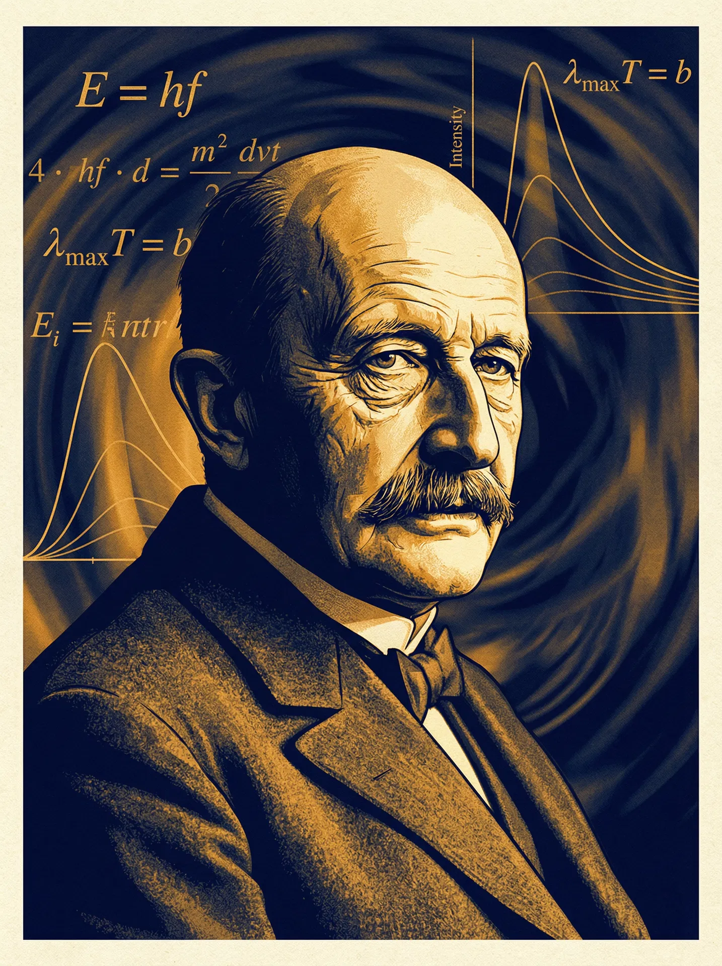
Max Planck
1858 – 1947
Father of Quantum Theory
- Solved the blackbody radiation puzzle (1900)
- Discovered that energy comes in tiny packets (quanta)
- Nobel Prize in Physics (1918)
- His formula is the starting point for all climate radiation calculations
Interactive Planck Curve
B(λ, T) — Blackbody Spectral RadianceDrag the slider to change temperature and observe how the blackbody spectrum shifts. Earth's surface temperature is approximately 288 K.
Karl Schwarzschild — How Radiation Travels Through Air
The equation that describes how heat is absorbed and re-emitted by gases
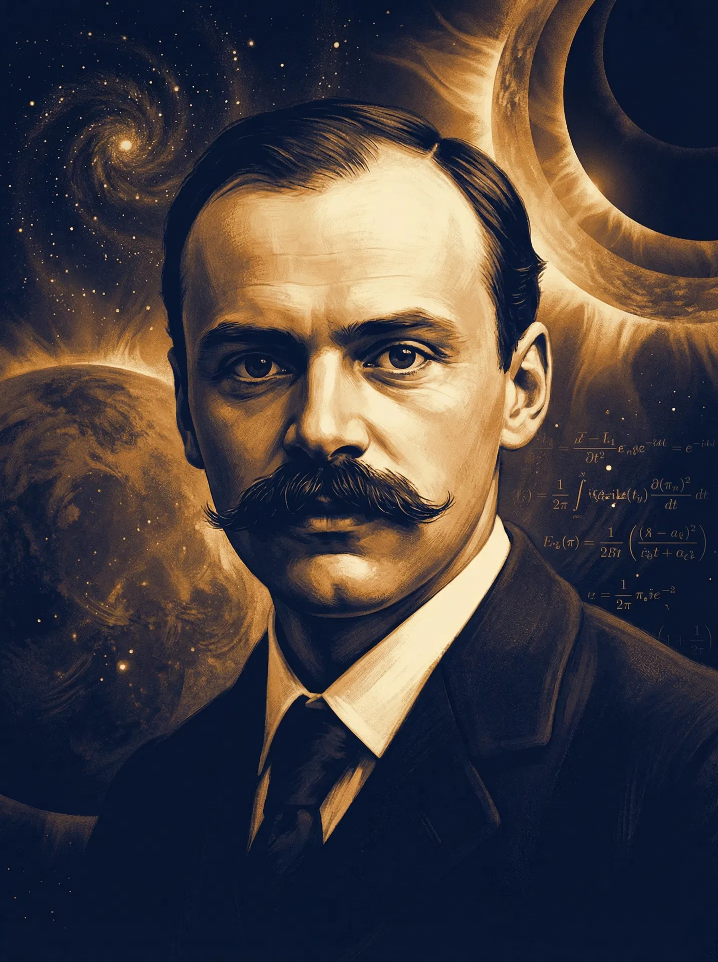
Karl Schwarzschild
1873 – 1916
Pioneer of Radiative Transfer
- Created the equation for radiation through gases (1906)
- His equation is used in every climate model today
- Also famous for black hole theory (general relativity)
- Died at age 42 while serving in WWI
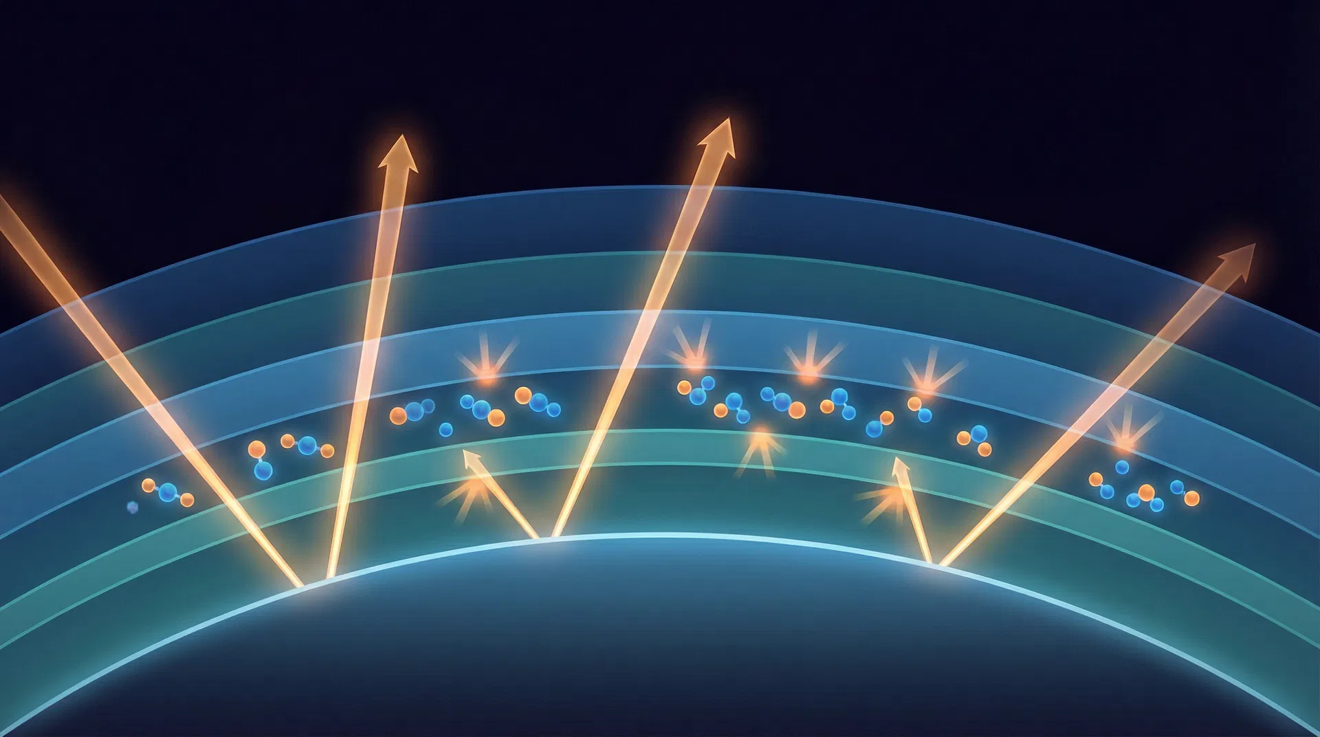
Planck's formula tells us how much heat a solid surface emits. But what happens to that radiation as it travels upward through the atmosphere? The air contains gas molecules (CO₂, water vapour, etc.) that absorb some of that radiation — and then re-emit it in all directions, including back down toward the surface. This is the greenhouse effect.
The German physicist and astronomer Karl Schwarzschild (1873–1916) figured out the mathematics for this process. While most people today know him for his work on black holes, his 1906 paper on the Sun's atmosphere is actually his most practically important contribution. He asked: if a beam of heat radiation passes through a layer of gas, how much gets absorbed and how much gets added by the gas's own thermal emission?
In plain language: As a beam of heat radiation passes through a thin layer of gas, two things happen simultaneously: the gas absorbs some of the incoming radiation, and the gas emits its own radiation (because it is warm too). The net change depends on whether the incoming beam is brighter or dimmer than what the gas itself would emit at its local temperature.
Why This Matters for the Chart
The jagged curves in the chart are produced by applying this equation step by step through the atmosphere — from the ground up to the top. At each tiny layer, the equation calculates how much radiation is absorbed and how much is added. The deep "bites" in the curve (around 667 cm⁻¹ for CO₂, and around 1595 cm⁻¹ for H₂O) are the frequencies where these gases absorb most strongly. The "window" region between 800–1200 cm⁻¹ is where the atmosphere is relatively transparent and most heat escapes directly to space.

The Chain of Influence
How equations designed for stars ended up in every climate model on Earth
The equations used to produce the chart were not originally created for climate science. They were developed by astrophysicists studying the Sun and stars. Over 120 years, a chain of scientists adapted and refined these tools until they became the foundation of modern climate modelling. Here is that chain:
Interactive Timeline
Click any event to explore the story — from quantum theory to modern climate charts
On December 14, 1900, Planck presented a groundbreaking idea: energy is not emitted smoothly like water from a tap, but in tiny packets called "quanta." This simple but radical idea solved a major puzzle in physics and launched an entirely new field — quantum mechanics. It also gave us the formula that tells us exactly how much heat radiation any warm object emits.
Annalen der Physik, 4, 553 (1901)
Conclusion
The spectral charts produced by modern researchers like Wijngaarden and Happer are not based on new or controversial physics. They are the direct result of applying two well-established equations — Planck's radiation law (1900) and the Schwarzschild equation (1906) — together with the precise molecular absorption data from the HITRAN database.
The story of atmospheric radiation science is a story of physics equations travelling across disciplines and centuries — from Planck's quantum revolution, through Schwarzschild's atmospheric equations, the astrophysical refinements of Eddington and Chandrasekhar, to the climate applications of Plass and Manabe. These equations remain as valid today as when they were first derived, and they are used by scientists on all sides of the climate debate.
We encourage you to explore the original papers linked in the References section below and form your own understanding of this fundamental science.
References
Click "View source" to access the original paper or resource.